Google Sheets is a service provided by Google that allows its users to assemble any kind of data in a neat and organized manner. It is especially used in the workplace where heaps of data have to be stored for decision-making purposes. However, if you have an entire Google Sheet full of data, the last thing you’d want to do would be to look at it and try to analyze it. No matter how organized it is, trying to make sense of the Google Sheet at the first glance can be quite difficult, not to mention intimidating.
If you want to understand your extensively filled Google Sheet within the first few seconds of looking at it, there is a perfect solution for you. This is where the Conditional Formatting Google Sheets feature comes in.
Contents
What is the Purpose of the Conditional Formatting Google Sheets Feature?
The Conditional Formatting Google Sheets feature is a visual organization feature that allows you to format your sheets’ cells according to certain conditions that you can define yourself. This allows users to change any, and all kinds of cell properties such as text color, highlights, cell colors, etc. based on their defined conditions or rules.
All these controls can make data stand out or be marked in a sea of filled cells, allowing the viewers to easily, and quickly, get the concepts of, or to take key information from, extensive data. This is also a great way to follow the progress of the task underworks and also to track goals.
Conditional Formatting Rules in Google Sheets
The Conditional Formatting Google Sheets feature works in a specific manner, meaning it follows a set of rules and a defined structure in order to carry out its intended function. Here is what you need to know about this feature before you dive into its working.
1. If/Then Condition
Every Conditional Formatting Google Sheets function works upon the if/then condition statement, which means that all conditionals follow the format “if this happens, then do that”
For example, if cell B5 is empty, then fill it with red color.
2. Conditional Formatting Structure
For the Conditional Formatting Google Sheets feature, a simple formatting system has to be followed that can be executed easily by understanding its three components, or key elements, according to which all the rules under this specific feature are structured. These key elements are:
a. Range: Range refers to the cell or cells that the rules of conditional formatting are to be applied to. For example, in the B5 example stated above, cell B5 is our range. This range can extend to multiple cells as well.
b. Trigger: Trigger refers to the cause that will result in the application of the conditional formatting rule. In our example, this is cell B5 being empty.
c. Style: Style refers to our command to Google Sheets that will be applied or executed if the trigger is satisfied. Here, in the discussed example, the style is the cell color being changed to red.
How to Use the Conditional Formatting Google Sheets Feature – Step by Step?
Applying Conditional Formatting to your data is inherently simple with the complications only increasing as we pile on the different kinds of Conditional Formatting options available. We can begin by talking about the basic steps with a simple example, then we’ll go into detail about the different kinds of Conditional Formatting options that Google Sheets offers its users.
For our first example of the Conditional Formatting Google Sheets feature, our condition will be to make sure that the cells are not empty, and based on this condition, the cells’ formatting will be changed.
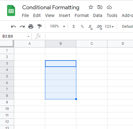
Step 1:
Select your range of cells. Here, we take the range B3 to B8 and select it. This method is suitable for smaller data sets; for larger data, you may input your range later.
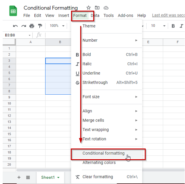
Step 2:
After selecting the data range, go to “Format” in the top menu bar, and then to “Conditional formatting” from the drop-down list.
Step 3:
A “Conditional format rules” dialog box should now show up on the right corner of your screen.
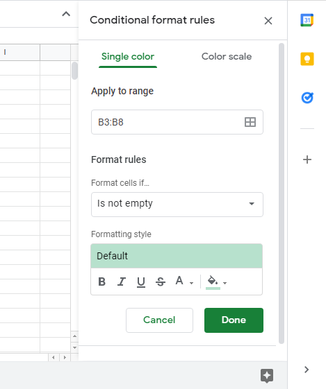
Here, as is visible, the Conditional Formatting Google Sheets feature offers a number of options. Let’s start with defining the conditions first, and then we will move on to further customizations based on the defined formulae (structure).
To define a trigger for your range, go to the “Format rules” section, and click on “Format cells if” to get a dropdown list.
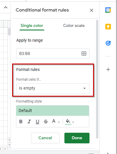
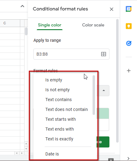
Here, you will get about 19 options. Since we’re only understanding the basics of the Conditional Formatting Google Sheets function for now, we will go with the first option that reads “Is empty”. Click on it.
Our trigger has now been defined. Since color is automatically defined by Google here, clicking “Done” right now would still get the job done.
Step 4:
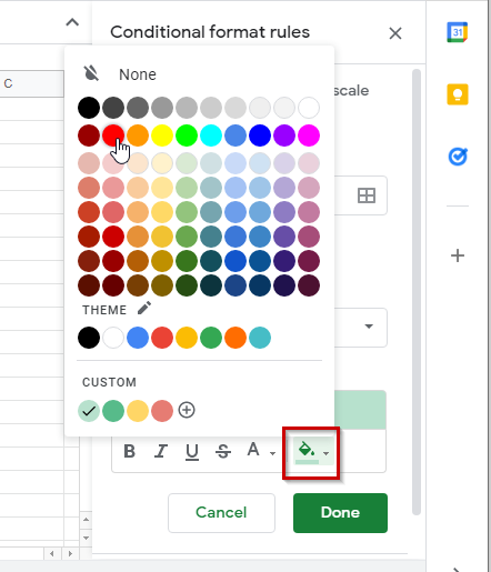
However, if you want to avail the option given you can alter the color of the cell highlight, and also the font specifics like bold, italicize, underline, overline, or text colors.
Since our condition is based on the trigger of the cell being empty, the only applicable customization option here is the cell color. Let’s set the style here which is to change the cell color to red.
Step 5:
Click “Done”.
Step 6:
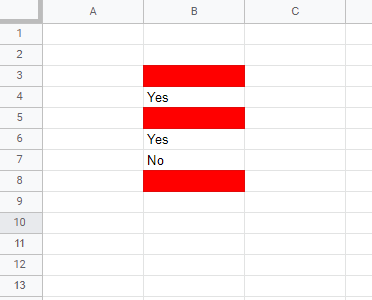
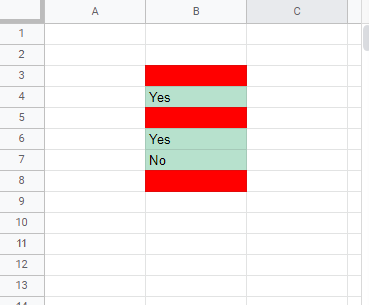
Now, to test the defined rule, enter some information in the cells from the defined range (B3 to B8). You can see here that since only cells B4, B6, and B7 have written text inside them, they are exempt from the red cell color. Conditional Formatting is, therefore, successful.
This is as simple as the Conditional Formatting Google Sheets tool can get, but there are heaps of options that for Conditional Formatting Google Sheets offers.
Types of Formatting Options for the Conditional Formatting Google Sheets Feature
There are many options that Google Sheets offers with regards to formatting rules, these can broadly be classified as those relating to cell blank vs non-blank states, texts, numbers, and dates. These are each discussed below:
1. Empty vs. Not Empty Conditions
Is empty: This rule will only be applied to your cell if the cell is empty. For example, the rule “If the cell is empty, highlight it red” will be followed.
Is not empty: This rule will only be applied to your cell if the cell is not empty. Let’s apply the rule “If the cell is not empty, highlight it green” to the previous example.
2. Text-Based Conditions
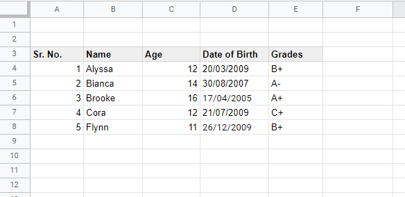
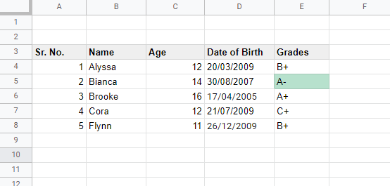
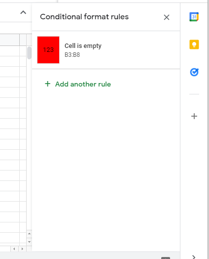
For individual text conditions, Google Sheets offers five different predefined settings. Here, let’s follow the example of a group of students, their names, ages, dates of birth, and grades listed against a column of serial numbers from 1 to 5.
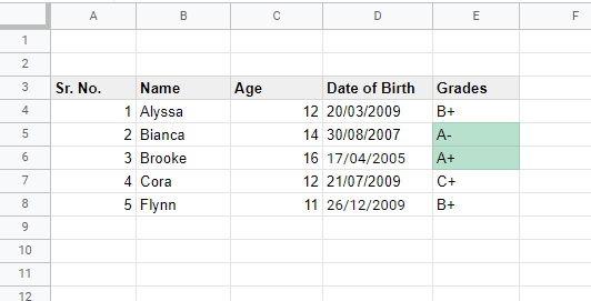
Text contains: This setting highlights an entire cell if the text or number in it contains the mentioned input anywhere in the text. Let’s highlight all the participants with A grades. Make sure to use the correct range which in this case is E4 to E8. 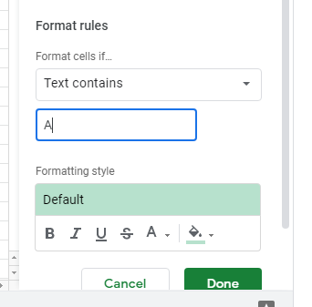
Shift the “Format cells if…” to the option of “Text contains”, and enter “A“ as shown above. You can then change the formatting style according to your requirements. Here, we are sticking with coloring the cell green. When selected, click “Done”.
Text does not contain: As is obvious from the name, this is going to exclude all the cells with the defined text. Let’s exclude the grades with the plus (+) now.
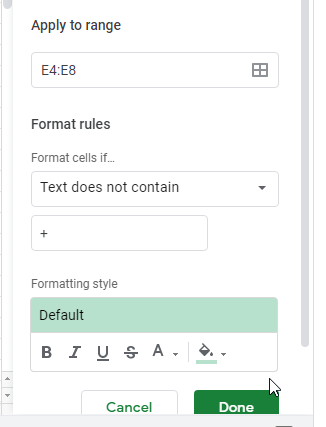
From the “Format rules” section in the dialog box, change the “Format cells if…” settings to “Text does not contain”. Underneath this box enter the plus (+) sign.
As can be seen here, Bianca’s were the only grades that did not have a plus (+) sign to them and so, this cell has been highlighted.
Text starts with: This setting highlights only those cells that start with a defined alphabet(/s), number(/s), or word. Let’s highlight the students whose names start with a “B”. For this, we are switching the original range and now have a new range that is B4 to B8.
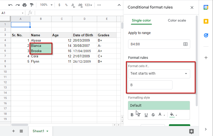
From the “Format rules” section, we will switch the “Format cells if…” settings to “Text starts with” and enter the alphabet “B” in the box underneath. If you wish to change the formatting style, you can do so now. Once everything has been sorted, click on “Done”.
Text ends with: This marks the cells ending with the defined criteria. To understand the “Text ends with” setting let’s highlight the birthdates of students born in 2009. This would again require us to change our range. The new range can be seen below:
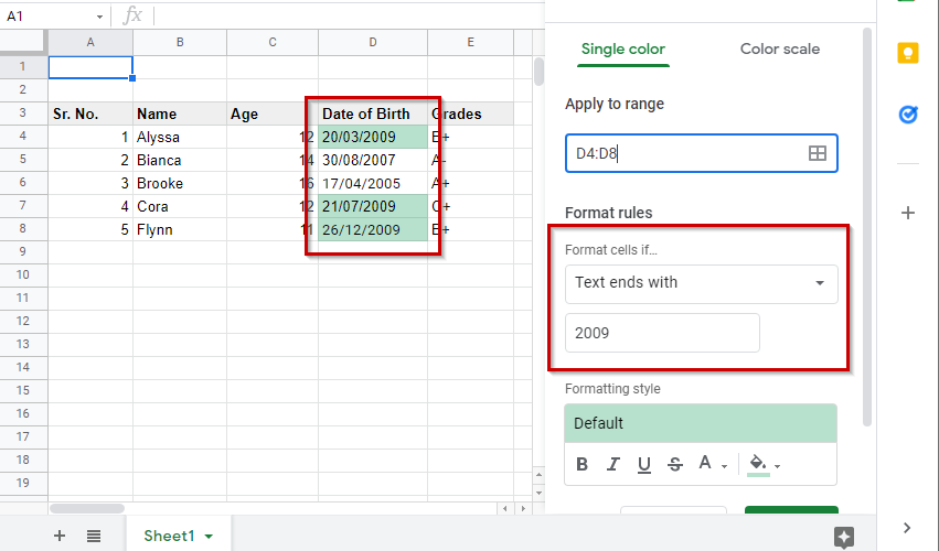
The formatting rules were changed accordingly and the “2009” was chosen as the ending text trigger. Afterward, we click “Done” to apply the Conditional Formatting Google Sheets feature over here.
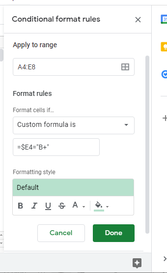
Text is exactly: This is going to look for the exact match in the range of cells defined. Let’s find grades that are “B+”.
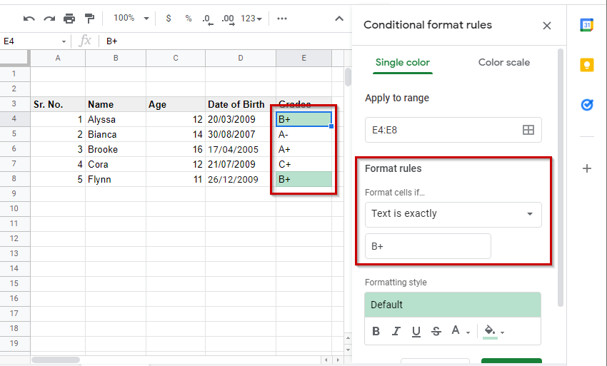
It is to be noted that in the case of writing “+” instead of “B+”, no cell will be highlighted in this Conditional Formatting Google Sheets condition.
2. Date-Based Conditions
For dates, there are three options offered by the Conditional Formatting Google Sheets feature. For each option, multiple specific options are offered as shown here:
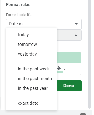
The three dates’ options are:
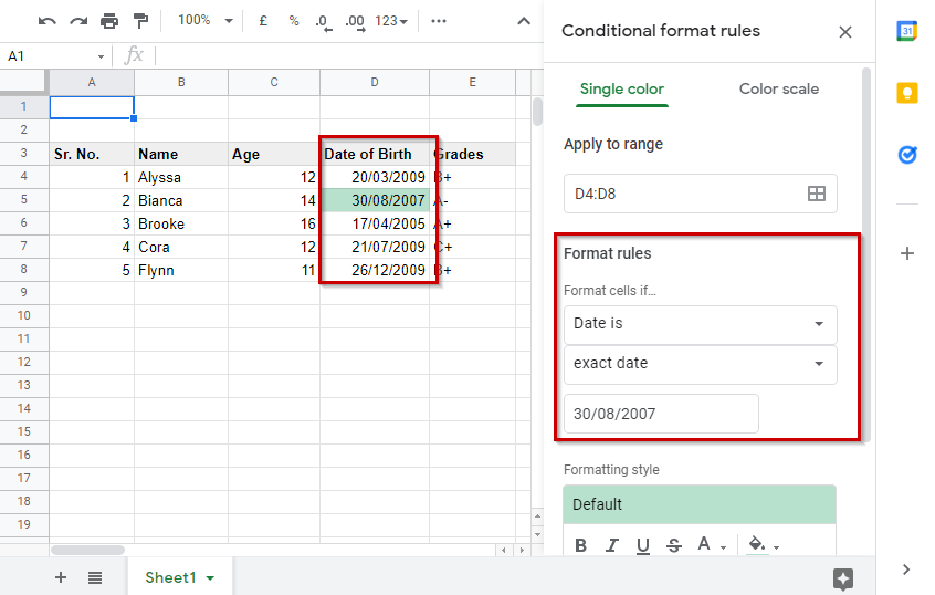
Date is: This is used to find a specific date. For example, here we are looking for the 30th of August, 2009. We have set the formatting rules according to our requirement of finding out an exact date.
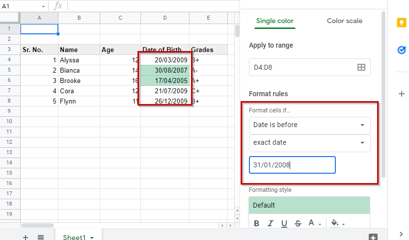
Date is before: This is used to highlights all cells/dates before a specified date. Let’s look for students born before the 31st of January, 2008.
Date is after: This is used to highlights all cells/dates after a specified date. Let’s look for students born after the 31st of January, 2008.
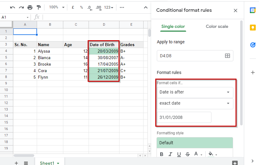
Tip: For date-based Conditional Formatting Google Sheets needs to have all the dates in the correct format.
For this, you need to make sure of two things. First off, make sure your dates are according to your Google Sheets’ locale. For example, if your input format is DD/MM/YYYY, and your locale is set to United States Google Sheets won’t consider it a date (since United States follows the MM/DD/YY format).
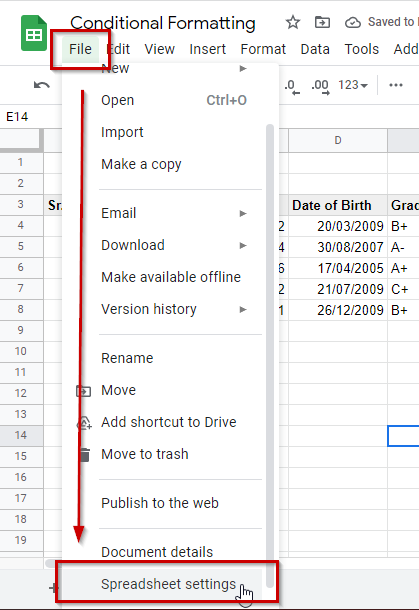
To make any changes in the Google Sheets’ locale, go to ”File”, and then to “Spreadsheet settings”.
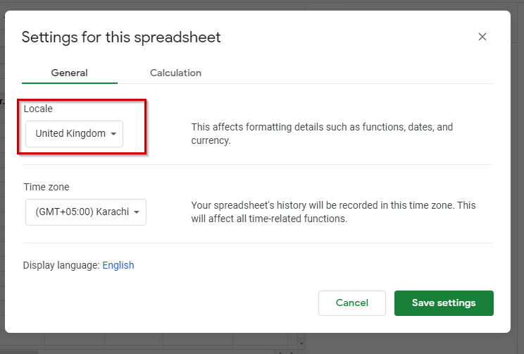
From the pop-up window make sure your Locale is set to UK for DD/MM/YYYY or US for MM/DD/YYYY. Choose your preferred setting and click on “Save settings”.
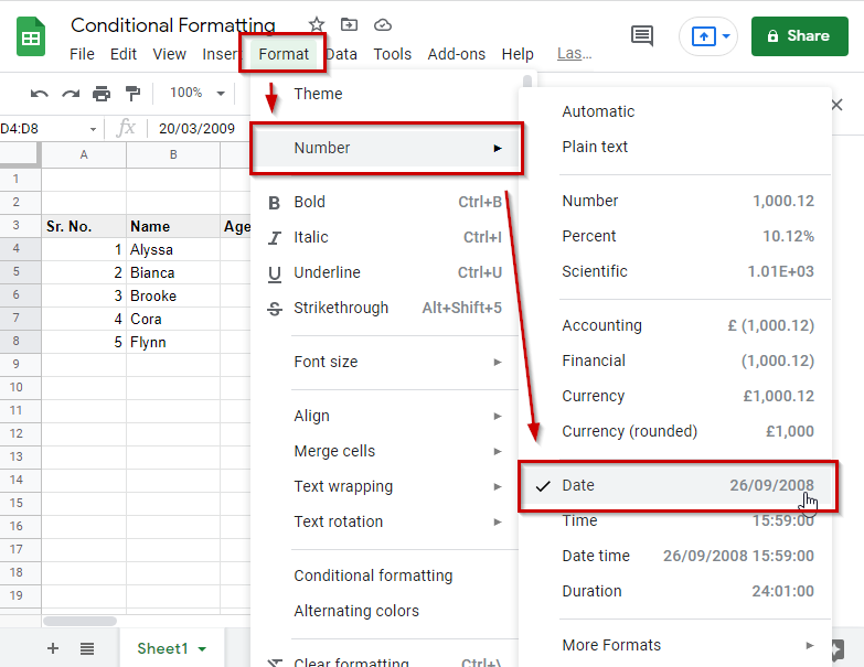
The second thing that you need to be sure of is that your dates are being read by google sheets as dates and not as random numerical values. For this, select the cell(/s) with the date(/s), and go to “Format”, and then to “Number” from the dropdown list, and then just make sure “Date” from the second list is checked.
Google Sheets often does this automatically, but in case it does not, now you know how to fix this small problem.
3. Number-Based Conditions
Eight different number-based settings are offered for google sheets conditional formatting.
These are:
- Greater than
- Greater than or equal to
- Less than
- Less than or equal to
- Is equal to
- Is not equal to
- Is between
- Is not between
All of these options are applied in the same way as the text and date settings. You just need to pick your desired formula type and enter in your specific numerical values. The Conditional Formatting Google Sheets feature will automatically understand it and produce for you, your desired result.
4. Custom Formula
The custom formula option allows users to make their own rules for conditional formatting. While this sounds complex, it really isn’t and is just the same as the other formulas for the most part.
The custom formula method can be used in several cases. Discussing the same example we have previously been using, if we want to highlight the entire data for the students born in 2009, or of those who scored B+, we can use the “Custom Formula” method to find the answer to this.
One important thing to understand for everyone wanting to use custom formulae in Google Sheets is that like every other Google Sheets formula, conditional formatting formulae also begin with the equal symbol (=).
Let’s take some examples now.
Custom Formula – Entire Row Formatting Based on One Condition
Let’s say you want to highlight the entire row for all students who scored B+.
Step 1:
Select the entire data range.
Step 2:
Or enter the data range manually. This will be A4:E8.
Step 3:
Select “Custom formula is” from the “Format cells if…” section, and in the blank space below enter =$E4=”B+”.
Here,
- “$E4” signifies all cells below cell E4 or all cells in column E starting from E4, and that our highlight will move along consecutive cells.
- “=” signifies the equivalence.
- “+B+”” refers to the equivalence being the string B+.
Step 4:
Adjust the formatting styles according to your preference. You can ask to change colors or any other font specifics.
Step 5:
Click “Done”. The sheet will now look like this.
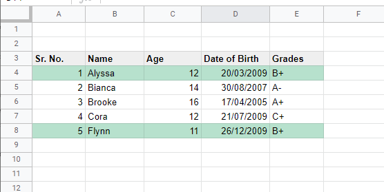
Custom Formula – Based on a Different Cell’s Value
Let’s say you want to highlight just the serial numbers of the students who scored a B+ grade. For this, you need to do the same steps as above, with a slight change in the formula.
Here, the formula will be
=E4=”B+”
Removing the “$” signals that the cell highlight is not to be made continuous over consecutive cells. The range will also be changed accordingly. The rest is the same.
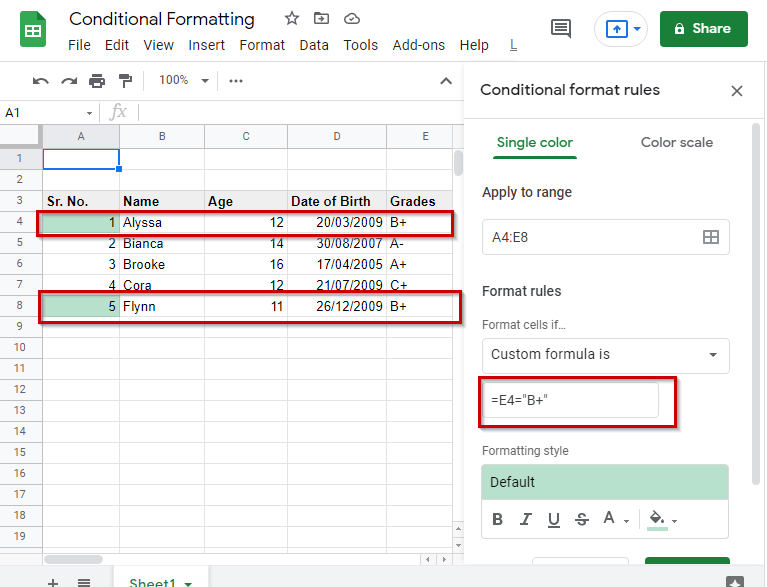
Custom Formula – Create your Own Multiple Rules at a Time
The Conditional Formatting Google Sheets feature can also be applied to multiple rules together, for one range of cells.
For this, click on any of the cells from the already defined range. If you’re starting afresh just go to Step 1 to define your first rule, first, and then start from here to add the second rule.
Clicking on any cell should open up this pop-up on the right side of the screen. However, if it does not show up, go to “Format”, and then to “Conditional formatting” again for it to show up.
Here, click on “+ Add another rule”, and then create your new rule.
Custom Formula – Highlighting Alternate Rows, or Columns
Through Conditional Formatting, Google Sheets offers a way to make zebra-like lines in your data. These are specifically useful for when one wants to read through large amounts of data. Besides making reading easier, these also make the data look more professional and refined.
To apply Conditional Formatting for this purpose, follow these steps:
Step 1: Select your range of cells.
Step 2: Go to “Format”, and then to “Conditional formatting”.
Step 3: The rest will be all as discussed above, and we will apply a custom formula here.
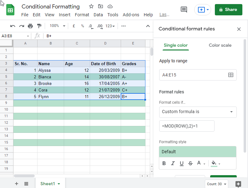
Select “Custom formula is” and enter in the formula “=MOD(ROW(),2)=1”
Here,
- “ROW()” refers to our rows.
- “MOD” is a function that divides the number of rows into two.
- “=1” means that when the remainder is 1 (odd row number) the row is highlighted. When the remainder is 0, (even row number) the row is not highlighted.
Step 4: Click “Done”.
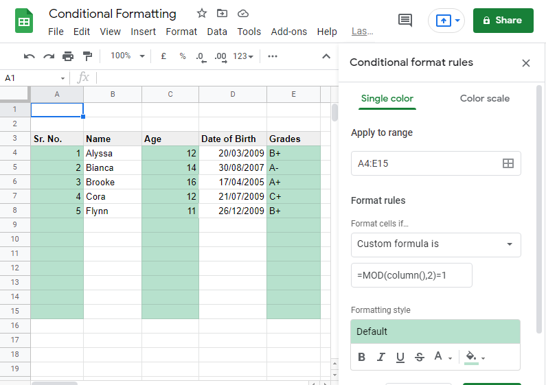
The same can be done with columns, by just going with the formula “=MOD(COLUMN(),2)=1”
Custom Formula – Color Scales
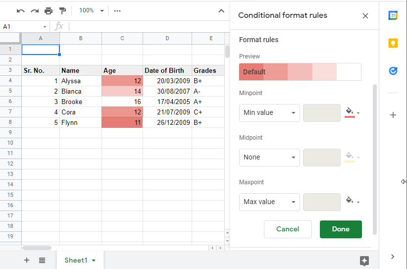
Making your highlighted text/cells fall on a range of colors depending on values is a very useful Conditional Formatting Google Sheets feature. This lets you represent your data that is in a range, to be represented on a gradient of colors ranging in hues or shades, according to values.
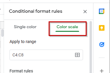
For example, let’s shade our participants’ grades on a gradient. Select your data range, and open the Conditional Formatting pop-up box. Click on “Color scale”
Here, the automatically selected limits or anchors are minimum to maximum values. However, you can choose from a number of different options according to your preference. Google will calculate and highlight accordingly.
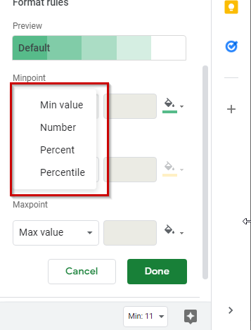
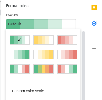
You can change the gradient colors by clicking on the colors’ preview, and can also customize the colors from the options available.
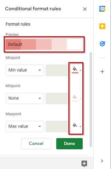
Once all the options have been selected, click on “Done”.
Your output will look like this now. White for “16” as it was for the maximum value, and the minimum value “11” has the darkest shade of the selected color gradient.