SUMIF Google Sheets – What it does, and how to use it?
 Image Source: Google
Google Sheets is a service offered by Google that allows users to create tables and spreadsheets. It allows users to store, edit, organize and ultimately analyze data in the most convenient manner. To make matters easier, it also offers a number of different functions and tools that help users deal with this data more easily and efficiently.
Unfortunately, most of these features offered are not used as often because most people find it intimidating to even begin trying. One of these features is the SUMIF Google Sheets function. As the name suggests, this feature is an amalgamation of the two separate SUM and IF functions.
The SUMIF Google Sheets function is a simple feature that scans through a range of cells of Google Sheets to find those values that match a given condition (the given condition being that of sum if XYZ condition is satisfied), and then once the match is found, the value listed in that cell (the one that matches the condition) is added to the group of selected numbers in the selected range. Once the SUMIF Google Sheets function is done scanning through all the cells in the range, it takes this whole group of selected numbers and sums them up!
Contents
SUMIF Google Sheets Function – Syntax
Each formula offered by Google Sheets carries its own syntax such as the VLOOKUP and the COUNTIF functions. The syntax for the SUMIF function is as follows:
=SUMIF (range, condition, [sum_range])
- Here “range” refers to the range of cells, inside which the function will be looking for the match to the given condition.
- The “condition” specifies the condition that is to be looked for and found positive in the specified range. It may be numbers, characters, range, or an alphanumerical string.
- Sum_range is optional. It specifies the range of cells from which the sum is to be calculated and is in correspondence with the range. In case sum_range is not specified, the sum will be calculated from values that match the given condition from the range.
How to use SUMIF Function in Google Sheets?
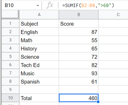
Let’s take a simple example of a student’s grades in seven subjects listed in column B inside cells from B2 to B8. “B2:B8” will be our range. Let’s say that we only want to sum up scores of subjects in which the student scored 60 or more marks, so our condition is “>=60”.
We will apply the formula and replace all variables with their appropriate terms:
=SUMIF (B2:B8, “>=60”)
Now, all the values from cell B2 to B8 that are greater than 60 will be added to calculate the results for SUMIF Google Sheets function in order to calculate the final grade.
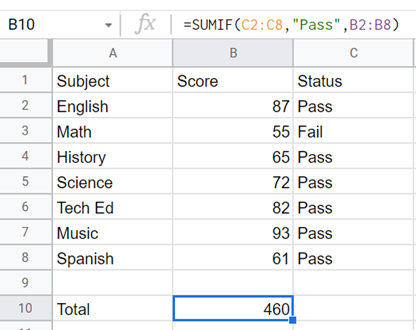
Let’s take another example with a specified sum_range. Here, we have a third column with the Pass/Fail remarks, and on the basis of this Pass/Fail status of the student in a certain subject we’re going to either consider or not consider that subject’s marks.
Here the formula will be:
=SUMIF (C2:C8, “Pass”, B2:B8)
Here, the range of cells has shifted from B2:B8 to C2:C8 because we are now concerned with the Pass/Fail status of the subject. This status will decide whether the subject scored will be added or not. The sum_range, however, is B2:B8 because the values to be added are present inside this range.
In this example, we have decided on the Pass/Fail status of the subject depending on whether or not the scores received are greater than (or equal to) 60 or not. We wish to add only the scores of the passing subjects hence the word “Pass” in the formula.
Where to Use SUMIF Google Sheets Function?
The SUMIF Google Sheets function is a versatile feature that can be used in a number of ways, and to accomplish a variety of different tasks. Some of the situations that it can be used for are:
- To find the sum of only positive or negative numbers
- To calculate salaries given to workers in one department
- To make student result cards
- To add the grade points (for finding average) of people in a certain age group, class, region, etc.
These applications are just some examples, and there are an infinite number of other situations and tasks that involve the use of the SUMIF Google Sheets function. The fact that it’s so easy to use is just an added bonus.
Using SUMIF Formula with Wildcard Characters in Google Sheets
The entire concept of wildcards is pretty convenient, not to mention easy to understand. A wildcard or a wildcard character is a special character that is used to replace one or more other characters when they are unknown or when we want to leave spaces for them. To use a wildcard character, it is to be written in the “condition” space of the formula.
By incorporating wildcard characters into your SUMIF syntax (into the condition portion of the function), the SUMIF Google Sheets function can be used in case we do not know the complete text or when we intend to match only a part of the text.
There are 2 wildcard characters commonly used for the SUMIF Google Sheets function. These are:
- Asterisk (*)
- Question Mark (?)
The “Asterisk” is used to replace a sequence of characters, whereas the question mark replaces one single character.
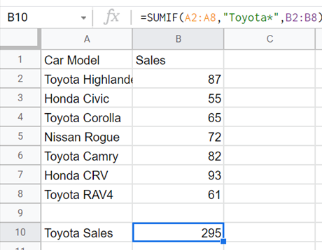
For example, from a list of cars for different companies, let’s find all from “Toyota” and add up their sales. Here, we will use the asterisk sign as the number of alphabets after Toyota is varying for all the different cars.
So,
The formula will be:
=SUMIF (A2:A8, “Toyota*”, B2:B8)
- Here A2:A8 is our range in which the “condition” is present.
- The condition is written as “Toyota*” as we have different Toyota models such as Toyota Highlander and Toyota Camry.
- B2:B8 is our sum_range which contains the sale numbers which are to be added up based on the given SUMIF condition.
How to use SUMIF for Different Data Types?
The variety of data types that can be used for comparison in the SUMIF Google Sheets formula for the condition argument is wide. We can use a wide range of data whether they be texts, numbers, or alphanumerical data. This would include dates as well.
Let’s break down these data types and discuss them in examples one by one.
1. Numbers
As mentioned in the first example, the SUMIF Google Sheets feature can be used to calculate grades, sales, percentages, etc.
The previously discussed example calculates sales based on the condition that all cars be from one company i.e., Toyota. It is going to ignore all other cells and will only take sales corresponding to cells that start from Toyota.
2. Alphabetical Data
The following example was also previously discussed where we calculated total marks based on the textual/alphabetical data given to us which was the status of the student in column C. Only those scores of the subjects were added that were passed by the student.
3. Date-Based Data
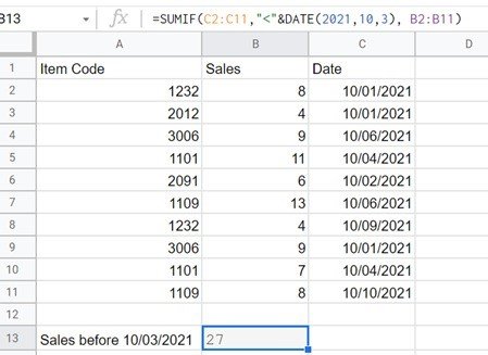
Here, let’s take an example of sales for different items made on random dates. Let’s find the sum of all sales made before the date 10/03/2021. In this condition, our SUMIF Google Sheets function will have to follow the following formula:
=SUMIF (C2:C11, “<”&DATE(2021, 10, 3), B2:B11)
- Here C2:C11 is our range for dates.
- “<”&DATE(2021, 10, 3) refers to dates before 10/03/2021
- B2:B11 are the cells with sales values to be added.
Range C2 to C11 is checked for the dates prior to 10/03/2021 and then, all the values from cell B2 to B11 for which the corresponding date in C2 to C11 is before October 3rd, 2021, are added to calculate the total sum. This sum (27) is then displayed in cell B10 in which we entered the SUMIF Google Sheets syntax.
SUMIF Google Sheets Function for Multiple Criteria
The SUMIF Google Sheets function has a limitation that allows it to only add values based on one condition only. However, if you want to base your results on multiple conditions, then all you have to do is simply add two or more SUMIF functions into one statement.
For example, to calculate the sum of Toyota and Honda sales together, we can use the formula:
=SUMIF (A2:A8, “Toyota*”, B2:B8) + SUMIF (A2:A8, “Honda*”, B2:B8)
Here we use two separate SUMIF statements and add in a + sign in-between.
Case-Sensitivity and SUMIF Google Sheets Function
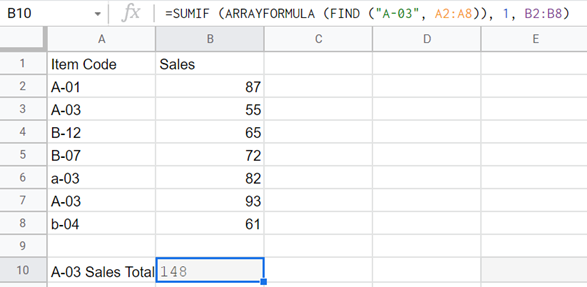
The SUMIF Google Sheets function, by default, is not case sensitive i.e., it does not see the difference between lower and upper-case letters. However, if you wish to manually make it case-sensitive and to identify uppercase and lowercase characters differently, you can use SUMIF in a combination with the FIND and ARRAYFORMULA functions.
The syntax will now be:
=SUMIF (ARRAYFORMULA (FIND (“text”, range)), 1, sum_range)
For example, let’s look for a specific alphanumeric keyword by using the following formula.
=SUMIF (ARRAYFORMULA (FIND (“A-03”, A2:A8)), 1, B2:B8)
In this example, the SUMIF function which is incorporated with FIND and ARRAYFORMULA function looks for “A-03” in range A2:A8 and returns the sum of its corresponding values from the range B2:B8, since it has been incorporated with FIND and ARRAYFORMULA functions, “A-03” will be case sensitive i.e., “a-03” will be not be counted.
SUMIF Google Sheets Function and Cells Being Blank vs Non-Blank
In some cases, we have to calculate sums on the basis of the corresponding cells being blank or non-blank. In such cases:
- “=” – Only blank cells are matched.
- “” – Blank cells and non-blank cells and zero-length strings are matched
- “<>” – Non-Blank cells including zero-length strings are matched
These are all mentioned in the condition argument.
Tips and Tricks to Remember While Using SUMIF Google Sheets Function
Here are some things that a user must keep in mind while using the SUMIF function on Google Sheets:
- When using the optional argument of sum_range, always make sure that both “range” and “sum_range” have an equal number of cells.
- It is essential to remember that the SUMIF function by default is not case-sensitive to avoid any errors, but if need be it can be made case-sensitive by incorporating FIND and ARRAYFORMULA functions.
- Numerals and cell references are not to be enclosed in quotation marks, while text value, data, and wildcards must be mentioned in quotation marks.
- If the condition consists of an operator and the cell reference or a function, the operator is to be enclosed in a question mark, and then they both ve to be joined using an ampersand (&) sign.
- Range and sum_range references cannot be substituted with arrays.
