
Google Sheets is a service offered by Google that allows users to create tables and spreadsheets. It allows users to store, edit, organize and ultimately analyze data in the most convenient manner. To make matters easier, it also offers a number of different functions and tools that help users deal with this data more easily and efficiently.
Unfortunately, most of these features offered are not used as often because most people find it intimidating to even begin trying. One of these features is the VLOOKUP Google Sheets function that we will discuss in this article. Created an extensive table and now need to find an unknown value in your table that corresponds to a known value? The VLOOKUP Google Sheets simplifies this digging for you.
Contents
What is the VLOOKUP Google Sheets Function?
The VLOOKUP Google Sheets function stands for Vertical Lookup. It is a frequently used search function in Google Sheets that allows the user to look up a value in a table and then to use it in another table, even when on a different sheet. It is used to search for a specific key, in a specific lookup column, in a specific table, and then to return the value that the user is looking for in the selected cell.
VLOOKUP Google Sheets – Formula
The formula for the VLOOKUP Google Sheets function takes 4 passing arguments i.e., Search Key, Range, Index, and Is_Sorted.
- Search Key denotes the key value or item that the user is looking for.
- Range indicates the range of cells that the value is to be searched for. For VLOOKUP Google Sheets, it may be a table or a column range.
- Index denotes the search column number, in the selected table, in which the user is looking for the specified value. For example, if you are looking at a table C3:F7, the single-column C will be numbered “1”. We do not use the column letter title system to denote columns for VLOOKUP. Columns D, E, and F will consequently be numbered 2, 3, and 4, respectively.
- Is_Sorted is to be used only when the user is looking for the closest match to the search key value. Commonly, users look for an exact match to the search key, instead of an approximate match, and the argument in such instances is set to FALSE. When you are more focused on similar matching instead, you would, however, change it to TRUE.
In case the user sets Is_Sorted to FALSE and none of the exact lookup values match, the VLOOKUP Google Sheets function will return “#N/A”.
VLOOKUP Google Sheets – Syntax
The syntax for the VLOOKUP Google Sheets command is fairly simple if you have understood the above-listed passing arguments well and their corresponding details.
The syntax for VLOOKUP in Google Sheets is:
=VLOOKUP (Search_Key, Range, Index, Is_Sorted)
For example,
=VLOOKUP (E5, A2:C6, 3, false)
Understanding the VLOOKUP Google Sheets Function – Example
1. Looking Up Exact Values
We will take the following data of some individuals, comprising their names, ages, and genders in a series, as our example:
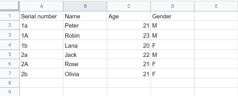
Now, let’s apply the function to this data set. First off, we need to pick a word that we are to search for in a specific column. For this example, let’s search for the word “Peter” here.
Step 1:
Write “Peter” in a cell e.g., A11.
Step 2:
Enter the formula =VLOOKUP (A11, B2:D7, 1, false) in a second cell e.g., B11.
Here,
- A11 is the cell with the word we want to search for.
- B2:D7 displays the range of cells of the entire table that can be screened by the VLOOKUP Google Sheets function.
- 1 is the lookup column. This means that the word “Peter” is to be searched for in the first column of the specified cell range.
- False dictates to VLOOKUP Google Sheets tool that we want to search for the exact word “Peter” and not a derivative of the word.
In the cell B11 (where the VLOOKUP formula was entered), Google Sheets will display the result.
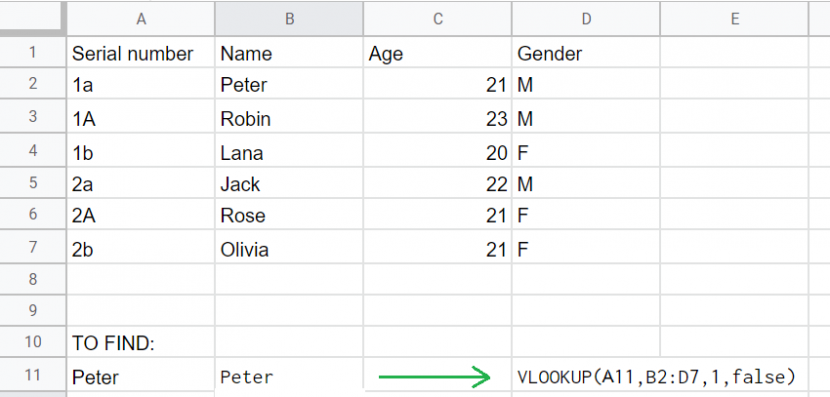
We can also do this by simply going with “Peter” in our formula instead of marking a special cell to be referenced in the formula. For example, we could have written “Peter”, instead of A11.
This means =VLOOKUP (A11, B2:D7, 1, false) is the same as =VLOOKUP (“Peter”, B2:D7, 1, false).
It must be made sure that if you decide to use letters in your syntax formula, you need to enclose the word in quotation marks.
2. Looking Up Corresponding Values
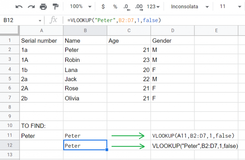
Let’s search for Peter’s age now. The syntax will be the same. The formula here will be =VLOOKUP (“Peter”, B2:D7, 2, false)
Here,
- Peter indicates the word that the VLOOKUP Google Sheets function needs to search for the corresponding value against.
- B2:D7 represents the table that VLOOKUP will scan.
- 2 indicates the column from which the corresponding value will be taken from. In this case, it is the second column of the specified table i.e., column C2.
- False dicates that the exact word “Peter” needs to be looked up and then consequently, the corresponding value.
This time our Index is 2 and we want to get returned a value from the adjacent column to that of the one containing our search key. The VLOOKUP Google Sheets tool here will give us the value, corresponding to Peter, from the second column which is the age column.

This example demonstrates how the indexes “1”, “2”, and “3” will return “Peter”, “21”, and “M”, respectively with the given table.
3. Looking Up Values that are Not Applicable or “#N/A”
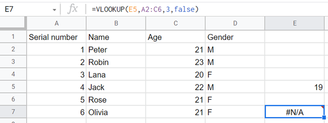
Let’s see what happens if we search for something that isn’t in our specified data. For example, let’s search for “19” in our list of ages.
The formula in this case will be =VLOOKUP (E5, A2:C6, 3, false). Here, the values that we have are,
- E5 is the cell containing the number that we want to search for i.e., 19.
- A2:C7 is the range of the table the VLOOKUP Google Sheets function will scan.
- 3 is the index number which is the column number that we are searching for 19 in.
- False represents that the user wants to search for the exact number 19, and not a number close to it.
Enter this formula, and the result will be displayed. Note that since the range has been changed from B2:D7 (in the previous examples) to A2:C7, the index for the age column has also been shifted from 2 to 3.
The result here, returned by google sheets, is an error message “#N/A” showing that our number “19” is not in the specified data range.
If we search for a value corresponding to 19, the same will be displayed as the table does not have “19” and therefore, no cell or value corresponds to it.
How to Use the VLOOKUP Google Sheets Tool on Separate Sheets?
For most of the spreadsheets that an average user comes across, the main table and the lookup table are on different sheets rather than on a single sheet. In such a case, for referring to the other sheet in the VLOOKUP formula we will put the worksheet name followed by an exclamation mark (!) before the range reference in the second argument, in the formula.
For example,
Sheet 1:
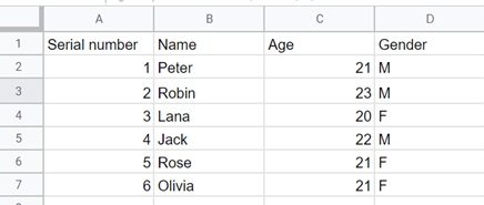
Sheet 2:
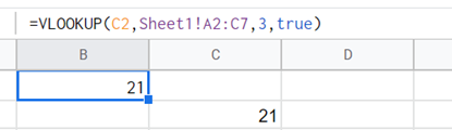
Here, we will use the formula, =VLOOKUP (C2, Sheet1! A2:C7, 3, true)
Google Sheets looks for the value, which in this case is “21”, in the cell references C2 to C7 (on sheet 1) and returns the closest match. Note here that instead of writing the age in a separate cell, we have directly referred to it from the original cell. This will also work.
VLOOKUP and Wildcard Characters
We can also use VLOOKUP Google Sheets to search for partial matches by using wildcard characters. Wildcard characters are special characters that are used to represent one or more characters. To use a wildcard character, we write it in the search key in the formula. There are 2 common wildcard characters used for VLOOKUP Google Sheets, these are:
- Asterisk (*)
- Question Mark (?)
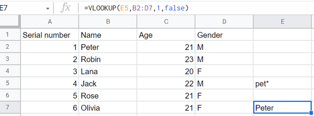
Asterisk is used when we want to match any sequence of characters. It is used on that specific side of the word on which the remaining characters are meant to be e.g., left or right.
For example, if we search for “Pet*” we will be returned with results that may be Pet, Pete, or Peter.
So, we write the formula =VLOOKUP (E5, B2:D7, 1, false)
Google Sheets will now look for the string in the name column (first key column of B2:D7 range) that has the characters “p”, “e”, and “t” in start together. As the word “Peter” starts with these letters, so replacing the asterisk (*) with “er”, the system returns “Peter”.
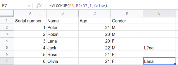
The question mark is used where we know the rest of the word but do not know one character. It is used as a replacement of the missing character.
For example, using the formula =VLOOKUP (E5, B2:D7, 1, false)
Google Sheets will look for the string in the name column (first column of B2:D7 range) that has the character L at the start then one random character followed by the set of letters “na”. as the word Lana starts with L and has “na” at the end with having only one character in between (“a” in this case), so replacing “?” with “a”, the system returns Lana.
In case you have an actual question mark as part of your search key content, then the wildcard character character “~” will be used.
Index Match formula for Left Lookup
A major limitation of the VLOOKUP Google Sheets function is that it cannot look at its left. In other words, if the search key is not found in a column in the lookup table, Google Sheets VLOOKUP will not look to its left one. In such a case, we can use another similar function that is more powerful and more durable i.e., the Index Match formula.
Its syntax is =INDEX (Return_range, MATCH (Search_key, Lookup_range, 0))
- INDEX is the name of the function that returns the value of a cell within the search range.
- Return_range is the corresponding range from where value will be returned.
- MATCH represents the function that represents the finding of a match of the search key in the lookup range.
- Search_key denotes the keyword or cell value that is going to be searched for in the specified table’s lookup range.
- Lookup_range is the range in which INDEX will search for a match for the search key.
- 0 is used to find an exact value in an unsorted table range. This is optional. We can either use 0 or 1. 1 is used to find the largest value that is less than or equal to the search key when the range is arranged in ascending order.
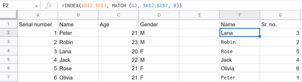
For example, if we want to find the names of people in the list, using their corresponding serial numbers, we use the formula =INDEX ($B$2: $B$7, MATCH (G2, $A$2: $A$7, 0))
Google Sheets here will look for serial no. 3 (mentioned in cell G2) from range A2:A7 and will return its corresponding name mentioned in the range B2:B7, which is Lana in this case. A similar process is repeated for all the cells from F3 to F7.
VLOOKUP Google Sheets and Case-Sensitivity
Sometimes we come across cases where the text case matters. As we know that VLOOKUP Google Sheets function is not case sensitive so we need an alternative, and thus, we use the INDEX MATCH function in combination with the TRUE function and the EXACT function to make a case-sensitive VLOOKUP Google Sheets array formula.
The syntax in this case will be =ArrayFormula (INDEX (Return_Range, MATCH (TRUE, EXACT (Lookup_Range, Search_Key), 0)))
- ArrayFormula is the function that is used to enclose a statement. It is optional, and the function(/s) will work the same with or without it.
- INDEX is the function that returns the value of a cell within the search range.
- Return_Range is the corresponding range from where the value will be returned.
- MATCH represents the function that will find a match of the search key in the lookup range
- TRUE dictates the MATCH function to return the first value it finds in the range, and won’t continue searching after that.
- EXACT has a similar purpose as that of MATCH but also differentiates between the uppercase and lowercase values from the column during the search.
- Lookup_Range is the range in which INDEX will search a match for the search key.
- Search_Key will represent the keyword or cell value that is going to be searched for in the specified table’s lookup range
- 0 finds an exact value in an unsorted range. This is optional. We can either use 0 or 1. 1 is used to find the largest value that is less than or equal to the search key when the range is arranged in ascending order.
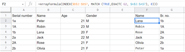
Applying this to a case sensitive serial numbers’ list, we use the formula =ArrayFormula(INDEX($B$2:$B$7, MATCH (TRUE,EXACT( G2, $A$2:$A$7), 0)))
Google Sheets will now look for the serial no. 1b (mentioned in cell G2) from range A2:A7 and returns its corresponding name mentioned in range B2:B7, which is Lana in this case.
A similar process is repeated for all the cells from F3 to F7. This can be done simply by selecting the F2 cell and dragging the selection down till F7.
Things to Consider when using the VLOOKUP Google Sheets Function
1. Case Sensitivity
VLOOKUP Google Sheets is not case sensitive i.e. it won’t be able to differentiate between upper case and lower case characters.
2. Looking for Exact and Similar Matches
VLOOKUP Google Sheets returns the nearest match when Is_Sorted is set to true, so if VLOOKUP is returning incorrect results, the user can set the Is_Sorted argument to FALSE so that it will return an exact match.
3. VLOOKUP and Wildcard Characters
The VLOOKUP Google Sheets function can search a value for a partial match by using a wildcard character. Wildcard characters are the asterisk (*) and question mark (?). A question mark (?) is used as a replacement of a single character in the range, while an asterisk (*) can be used to match a sequence of characters from the range.
Frequently Asked Questions (FAQs)
Q. What to do if I want to look up data horizontally?
Ans. For a horizontal lookup, google sheets offers another function called HLOOKUP.
Q. How can I get rid of the “#N/A” error?
Ans. In order to run your function smoothly, the most important thing is to make sure the formula values are set up correctly. If you have effectively made sure that your formula is wholly entirely free then the probable reason for your error is the absence of the referenced lookup value in your data.
Q. What can I do if I’m confused about errors and the absence of lookup value?
Ans. For confusions like this, there is a function called IFERROR in Google sheets. This function gives you a zero “0” if your formula has an error, otherwise displays the result. The syntax for this function is =IFERROR (FORMULA(), 0 )).