
In this article, we will teach you how to merge cells in google sheets which will add to the aesthetic appeal of the document and also make the document easier to understand by your professional peers.
Google offers a wide range of applications for our academic and personal needs. It is necessary that we understand how these applications work to be able to produce a document that not only provides us with the necessary information but is also appealing to look at.
Done organizing your data on google sheets? But hey, it looks like your google sheets’ tables have some cells with repeating texts that would ideally look better arranged some other way.
It looks okay and works alright, but there is a simple way to make your google document look better and more refined, and that is to merge such cells, avoiding repetition.
To make your work easier for you, we have a step-by-step guide that answers and covers all your probable questions and issues.
We will be discussing the steps involved to merge cells on google sheets for not only the desktop version of the Google Sheets application but also the mobile version.
Starting off with the desktop version, all required steps have been discussed below in detail:
Contents
How to Merge Cells in Google Sheets on Desktop
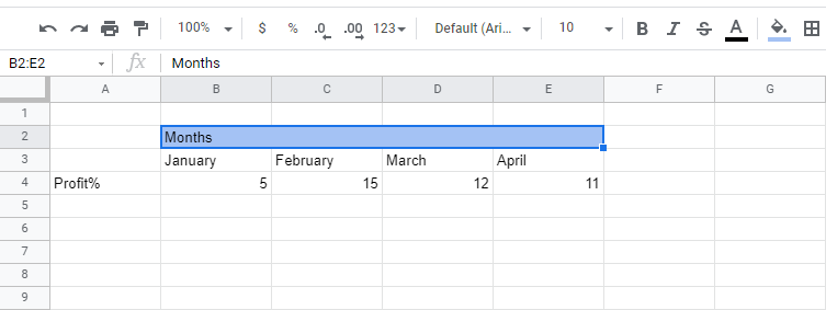
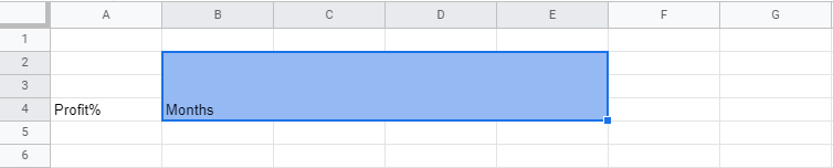
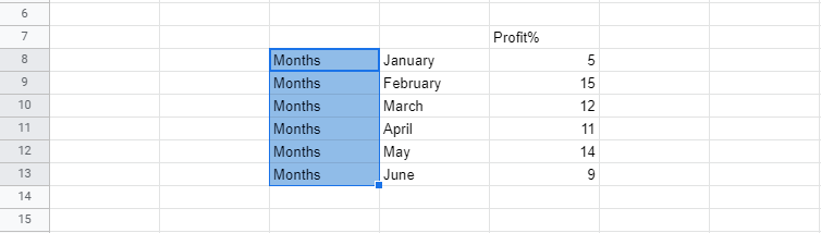
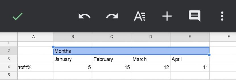
Starting off with this table as an example.
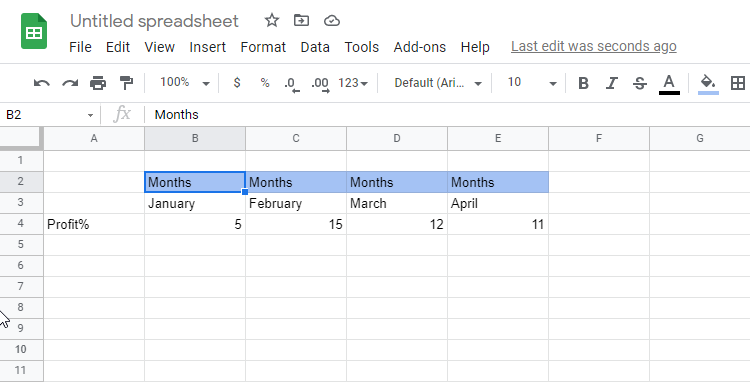
In this example, we want to avoid the repeated usage of “Months”, and to merge all the cells, that read “Months”, into one, producing a header row.
Now there are two ways to merge your cells in google sheets, and we’ll go through both of them step-by-step.
The two methods differ by the menu option selection on the spreadsheet viz. It could either be the worded menu with “File”, “Edit”, “View” etc. placed side-by-side or the icons’ one that runs immediately below.
First Method; Worded Menu:
To elaborate better on the method we are talking about, here’s an image highlighting the menu to be used:

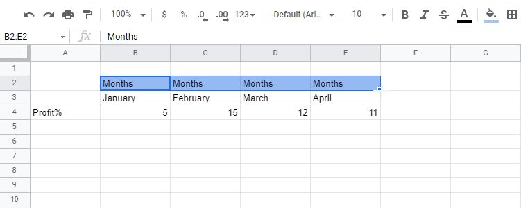
Step 1: The first step in either of the method employed would be to collectively highlight the row, the column or any arrangement of cells that are located adjacently, you need to merge. Here, we have added an example where a row of cells is highlighted.
Step 2: From the menu in consideration, we will use the format option.

Step 3: Clicking on “Format” will extend a drop-down menu/list. From this drop-down list, go to the “Merge Cells” option and click on it.
Step 4: Click on the “Merge horizontally” option.
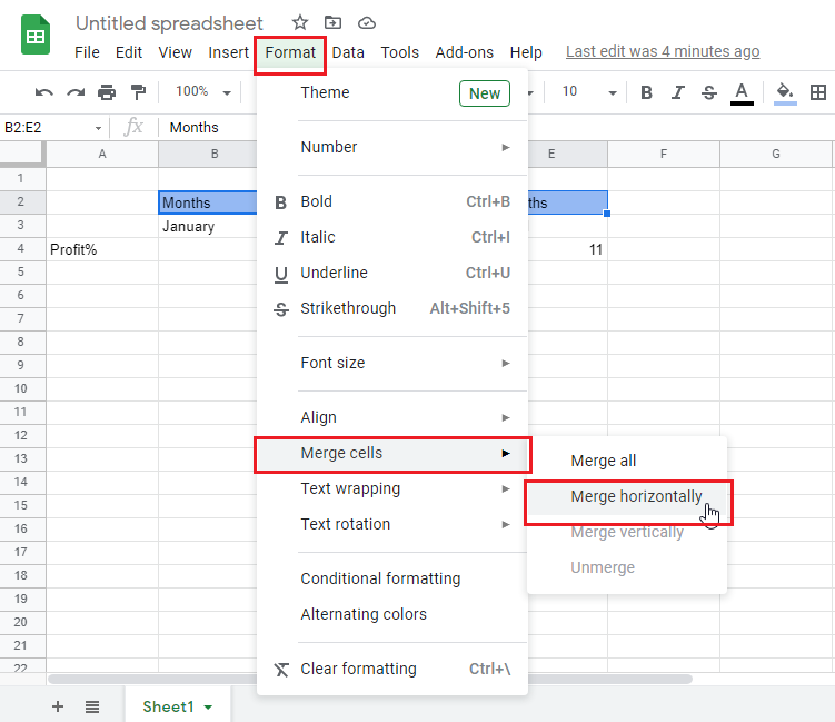
It is to be noted here that this decision of either selecting the “Merge horizontally” option or the other two will depend on the arrangement of original highlighted cells. There will be a detailed discussion on these options in subsequent segments of this article.
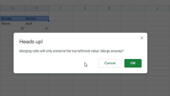
Step 5: Upon receiving the following question, click “OK”.
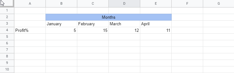
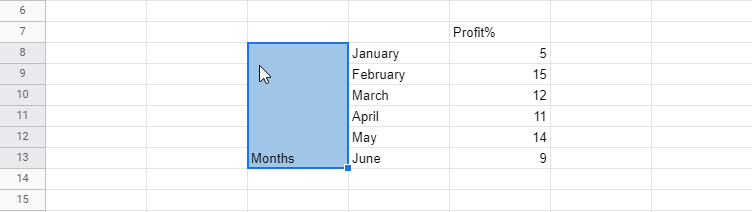
The table will now look like this.
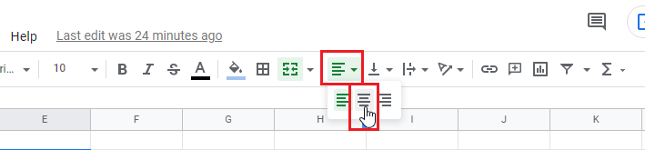
Step 6: To align the text to the center which is now a one single cell, go to the alignment option in the icons’ bar and then click the center alignment option.
The table will finally look like this, and your alignment is done making your google sheets document look much more efficient.
For vertical alignment (in the case of column cells) to the center, go to “Format”, ” Align”, and then click “Middle”. Vertical Alignment scenario is further explained in detail later in this article.
Second Method; Icons’ Menu:
For the second method, we will use the second spreadsheet menu or the toolbar characterized by its distinct way of using icons instead of fully formed words.
Step 1: The first step would be the same which is to select all the cells to be merged.
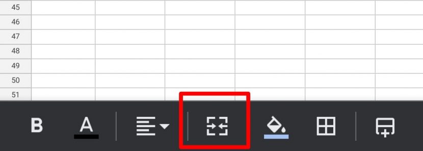
Step 2: Then go to the merge option on the toolbar and click on it.

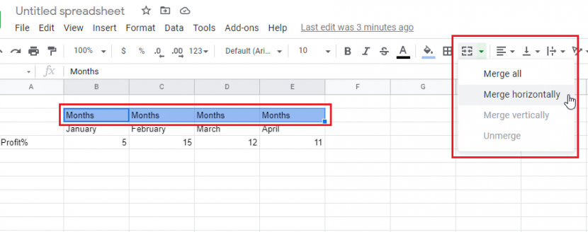
Step 3 (Optional): Clicking on it will automatically merge the cells, however, if you click on the dropdown option, you will get certain options to pick from.
The alignment can be adjusted in the same way as was discussed for the previous method.
Options Offered for Merging Cells in Google Sheets
Now that we’ve discussed the basic methods, we move on to the different options you get related to merging your cells in google sheets. When you try to merge your cells, you are presented with four options. These are:
- Merge all
- Merge Horizontally
- Merge Vertically
- Unmerge
Merge All:
This one entirely depends on your selection of table cells. Whatever cells you select, it will make sure to merge them, with the content of the top, leftmost, or the top-left cell being preserved. You simply select any or the entire range of cells to be merged into one and go to the “Merge all” option button to merge your cells.
Here is an example indicating the before and after of Merge All type in google sheets.
Before:

After:
Here as you can see the entire table’s cells have been merged and for this one cell “Months” is preserved only with the other cells’ contents being deleted. For further refinement, you can use the center alignment option to carefully fit the word “Months” to the center of the new cell.
Merge Horizontally:
“Merge Horizontally” only merges horizontally selected cells, that are in a row. This is just like the previously discussed main example. Select your horizontal cell range and go to the merge horizontally option. The data in the left cell will be preserved.
Before:
After:
Merge Vertically:
As is obvious from the title, this option helps you in merging vertical cells, that are in a column. Select your vertical cells and go to the merge vertically option. The top cell’s content will be preserved.
This will be your before and after.
Before:
After:
The method of middle alignment from the “Format” option can be used to bring the cell content up to the middle for a better visual effect.
Unmerge:
To unmerge your merged cells, simply select the merged cell and either tap on the merge icon in the icons’ toolbar, or go to “Format”, “Merge Cells”, and then “Unmerge”.
How to Merge Cells in Google Sheets on Mobile
The process of merging cells on mobile on google sheets is easier than that on the desktop version.
Step 1: Again, beginning with the common step which is to select your cells.
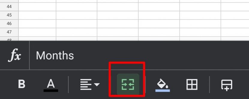
Step 2: Once your desired cells have been selected, the next step is to click on the merge icon. The configuration of your phone’s google sheets application will be different depending on the type of phone you own (Apple, Android).
And there you have it. With just two steps you have successfully merged your cells.
This one icon will merge your cells whether they’re vertically selected or horizontally selected, or are in both directions. Just like it is for the “Merge All” option on your desktop, you select your entire cell range on the mobile and go to the merge cells option.
Step 3: Now familiar to us is the concept of center alignment, which we can use to bring the text to the center of the cell. The icon for this has been shown in the above image to the immediate left of the merge icon.
Step 4 (Optional): To unmerge, simply select your merged cell, and tap on the merge button again.
The image below shows that the cell selected currently contains the word “Months”.
Potential Issues for when you Merge Cells in Google Sheets
While google sheets is a great tool for one too many things, it also has its limitations, and when you have merged some cells on the tool you might encounter some issues while working on your sheet. Such potential issues are discussed right on.
Sorting Columns with Merged Cells:
Managing or working with a column in which you have some cells merged can give errors or be bothersome. Sorting out such columns is important for analytics, and if columns with merged cells are bothersome to sort, you may have to sort them manually with potentially having to unmerge your cells temporarily which is time taking.
To avoid this you may have to make sure to perform analytics in separate columns from the merged cells to avoid going back and forth on the single column you are working on.
Selecting Cells from an Assortment of Merged Cells:
Simply selecting a select few cells from a series of merged cells is not possible, and if you try to select such cells, the merged cell, as a whole will get selected. This again might make you have to unmerge cells on your google sheets document to continue your work, thereby, wasting your time.
This applies both to columns and rows – vertical and horizontal cells.
Copy-Pasting Data off Merged Cells:
Trying to move your data by copy-pasting it to a different location is not possible with merged cells, as it will also copy and paste the formatting of the merged cell or cells to the new or second location. In order to copy the cell content, you will have to copy solely the value of the individual cells e.g., from the formula bar.
Frequently Asked Questions (FAQs):
Q. What is the shortcut for merge cells in Google Sheets?
A: You may use the following shortcuts for Mac and Windows:
Mac: Ctrl + Option + O, M , Enter
Windows: Alt + O, M , Enter
Q. Can you merge entire rows or columns?
A. Yes, to merge two or more entire rows or columns simply select the row headings (e.g., 1, 2, 3, etc.) or column headings (e.g., A, B, C, etc.) and click the merge icon.
Q. How to find merged cells in google sheets?
A. A simple method to find merged cells in your google sheets document is to go to “Format”, and then to “Conditional Formatting”. Here, under the rules and already picked single color option, set up the Range as “A1:Z1000” and custom formula to “=MOD(ROW(),2)=0” for rows and click done. Do this again with the formula “=MOD(COLUMN(),2)=0” for columns. Now you can look for your merged cells.
RELATED POSTS